My Master’s
Well, these two last weeks has been to busy to my taste!
For those who don’t know me, I’ve started my masters as a special student in UNESP Brazil last semester. It was a really nice period of much knowledge in computer science, a lot of work, research tests and sweat.
When I was about to start as a “special student”, I was allowed to choose only for two different subjects at most. Since my thesis would need deep knowledge on algorithms and high performance computing (HPC), I was planning to take classes on these topics. However, the HPC classes schedule was not the best for me, so I started looking for something else. There were plenty of good options including AI, computer vision, databases, etc. Choosing the best one for me was hard as chase a chicken.
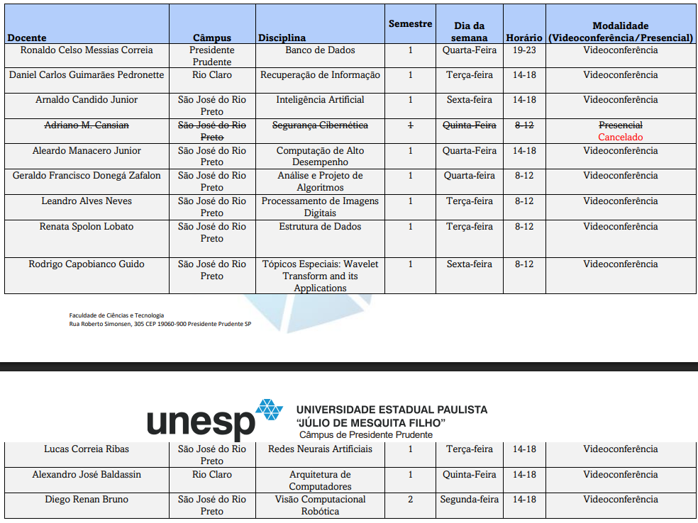
However, in the list there was something really different to me. Most part of the subjects names were written in portuguese, well all but one. This one was named “Wavelets Transform and its applications”. I had never ever heard about wavelets. I googled it a bit and saw some relation with Digital Signal processing (DSP) and some people talking the relation wit Fourier Transform.
I had some previous knowledge on Fourier Transform, since the courses and lecture notes I took on quantum computing had the quantum relative, and because 3Blue1Brown did a great job on his video.
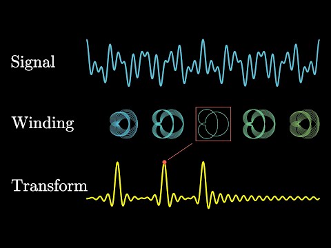
Besides that, FT was much more like a thing that I had heard but never actually used in something mine.
Well, but at that moment, I knew that something interesting could be extracted from it, so I decided to apply for this class.
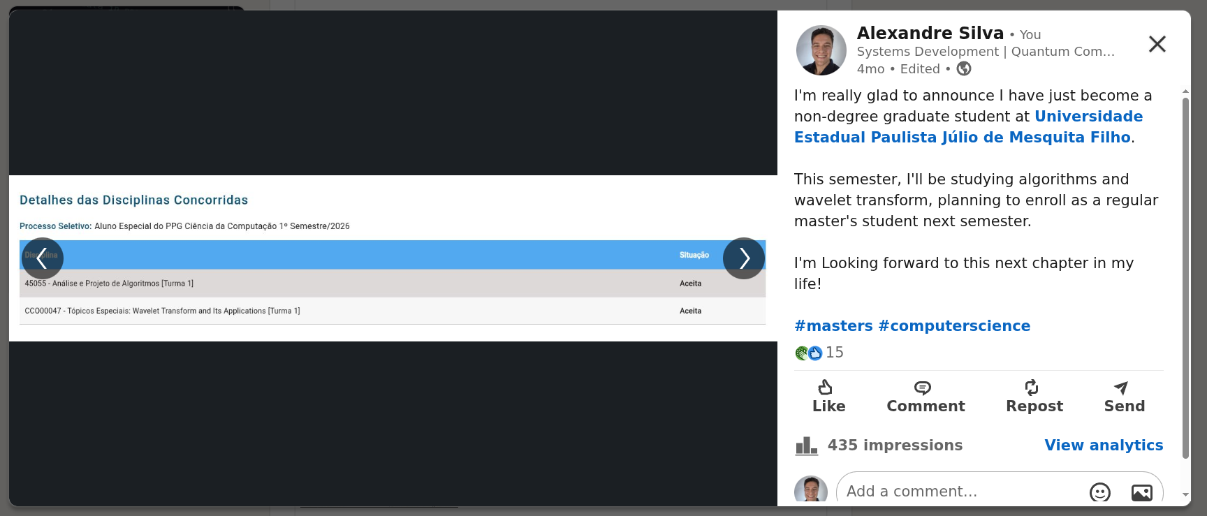
My final choices was algorithms and wavelets. The first one I knew I was going to be accepted, since the professor happened to also be my advisor in my masters. But the other one, I was pretty nervous and anxious for the result. But thank god, it happened and both accepted me, so that was my first step.
Final projects
Well, six months has passed and we finished our classes.
During our classes on algorithms, we learned a lot about complexity and algorithms in general, but the main focus was in sorting algorithms both using primary (RAM) and secondary memory (HDD). It was pretty nice, since I thought the previous course I had took on the topic had some lacunes, but this one has fulfilled them. For this course we had to give a seminar and write a paper in some topic we would like to explore and give algorithm analysis about it. The topic I chose was “quantum circuit simulation using tensor networks”. It was kinda new to me, but I’ve learned a lot in the process.
I had never dived into such a topic like this, so it was nice to me. I learned a lot about tensor networks, hypergraphs, hypergraph partitioning, and many others. The algorithms I chose to analyze was PHyper-Par from withtin the Cotengra framework. For interested readers, the original paper can be found here. I also had to analyze the KaHyPar algorithm, which is used by Hyper-Par for hypergraph partitioning, the paper can also be found here.
The paper I produced is in progress to be published so you’ll probably see more in the near future. For now, people interested in my project can take a peek by looking at the resources and the research materials in my github repo at https://github.com/Dpbm/mestrado-aulas/tree/main/algoritmos/projeto-seminario. At the moment I wrote this article I also found many different interesting resources which I’ll list bellow.
- https://github.com/kahypar
- https://docs.rs/mt-kahypar/latest/mt_kahypar/
- Scalable Shared-Memory Hypergraph Partitioning
Now, for the Wavelets course, it was a little bit more easygoing that the other. Every week we had our classes and then we a homework activity. At the end, he gave us a small test, which was in general a set of exercises to be done whithin some weeks and then handed in until July 3th. The exercises covered most part of the topics we have studied until the date he handed out, so lots of cool things, such as DTWTs 2D-DWT, DTWPT, finding some equations, etc. It was really nice.
Since our professor allowed us to do the way we found it better, once the goal of the course was to give us the tools not to deep dive into wavelets mathematical concepts, we could do the things with software. I decided to do it by hand and test it with software, just to ensure the answers were correct. At first, I used a combination of 3 tools: PyWavelets, SymPy and Numpy.
Using Sympy
The simpler execises were easy to test using Sympy and Numpy. We only needed to generate the matrices using the Matrix class from Sympy and apply a dot product using * operator and pprint() to nicely print the output.
# Example sympy for Inverse DTWT

from sympy import simplify, Matrix, pprint

h = [
# low pass filter
]
g = [
# high pass filter
]

m = Matrix([
        [h[0],g[0],h[2],g[2]],
        [h[1],g[1],h[3],g[3]],
        [h[2],g[2],h[0],g[0]],
        [h[3],g[3],h[1],g[1]],
    ])

v = Matrix([
# coefficients
    ])


pprint(simplify(m * v))
I’m not sure if I could provide the results I’ve got and the code I used online, since my professor may use the same material in the future. So, I’m not sharing it on my github. Altought, I can provide some interesting things I found in the meanwhile. Also, even though the code I used could not be shared, some notes and tests I did durig the course are also available on my Github at https://github.com/Dpbm/mestrado-aulas/tree/main/wavelet.
Simpy is a pretty nice tool that everybody should use at some moment for mathematical equations. It features an amazing syntax, which is pretty much the same API as Numpy, which a few nuances.

While I was doing this exam, I discovered some things that might be valuable for you in the future. For a more experienced Sympy user, this might seem a usual thing, but since it was my first time I found it interesting.
So, in general, while computing those matrices with Mallat’s algorithm, we usually want a simple coefficient, not in decimal by not too extensive. Sympy usually simplifies the maximum it can do, which sometimes was not the best for my case. To overcome this problem, I took two different approaches. At first I used the cancel() function instead of simplify(), it worked in some cases, but again there was a lot of moments that It was not enogh. So the overall best case for me was to join fractions myself. It was not hard since the coefficients were simple, so multiplying a side by $2/2$, $4/4$ or $8/8$ was the best in this case.
I searched if there were some other approaches but the best I could find was to turn of the evaluation while computing the dot product:
from sympy import pprint, evaluate

with evaluate(False):
    a = #... the dot product ....
pprint(a)
For me it was not sufficient as well, but it helped me sometimes when I needed to debug some things.
When you compute a dot product without evaluation in sympy, it’s straightforward to understand which coeffients are being used for each cell, so it came in handy in some of the exercicies, chiefly in those involving inverse DTWT, where I accidently misplaced filter coefficients 😅. It’s always good to remember that the $h[2]$ and $g[2]$ come first than $h[3]$ and $g[3]$.
# CORRECT
m = Matrix([
        [h[0],g[0],h[2],g[2]],
        [h[1],g[1],h[3],g[3]],
        [h[2],g[2],h[0],g[0]],
        [h[3],g[3],h[1],g[1]],
    ])

# WRONG
m = Matrix([
        [h[0],g[0],h[3],g[3]],
        [h[1],g[1],h[2],g[2]],
        [h[2],g[2],h[0],g[0]],
        [h[3],g[3],h[1],g[1]],
    ])
Anyways, it was nice to play a bit with it.
Using PyWavelets
For more compelex exercises, such those requiring 2D-DWPT, I tried using PyWavelets.
This is another amazing python library that you should try. However, there are some big nuances you should now first.
- There’s no trend of fluctuation in this library. Some portion of the wavelets literature use approximation for low-frequency portion and detail for high-frequency portion, in our case they are relatives to trend and fluctuation respectively. If you want to be sure the coefficients you are using you can use some code like this to verify if the values match the expected:
import pywt

# example Daubechies: vanishing moments=2, support size=4
db = pywt.Wavelet("db2")

print("Decomposition (analysis)")
print("trend: ", db.dec_lo)
print("fluctuation: ", db.dec_hi)

print("-"*30)

print("Reconstruction (synthesis)")
print("trend: ", db.rec_lo)
print("fluctuation: ", db.rec_hi)
- All values are normalized. I cannot say for sure what’s the values for each one, but for Daub-2 the filters coefficients were weighted by $\frac{1}{\sqrt{2}}$, so to get the values as usual you should multiply the values by $\sqrt{2}$.
import pywt
import numpy as np

# example Daubechies: vanishing moments=2, support size=4
db = pywt.Wavelet("db2")

print("Decomposition (analysis)")
print("trend: ", np.array(db.dec_lo) * np.sqrt(2))
print("fluctuation: ", np.array(db.dec_hi) * np.sqrt(2))

print("-"*30)

print("Reconstruction (synthesis)")
print("trend: ", np.array(db.rec_lo) * np.sqrt(2))
print("fluctuation: ", np.array(db.rec_hi) * np.sqrt(2))
It seems like Decomposition and Reconstruction are flipped. While I was testing the results, I found that the reconstruction was acting as decomposition and vice-versa. I’m not sure if I was wrong in some way, but found it a bit confusing. So in my tests I just used it flipped.
They may not be using Mallat’s algorithm for the calculations. I was doing the 2D-DWPT for one of the exercises, and for some reason the values were too off to what I was expecting (I was using the builtin dwt2 methods). I tested many things, even used Chatgpt to help me understand the problem. At end, I understood that they were not using the regular Mallat’s algorithm, so even though the answer was pretty much the same, the step-by-step was different, so it only made more confused.
To solve that, I decided to take a step back and use the regular Sympy approach such as in the following:
import numpy as np
from sympy import simplify, Matrix, pprint

s = Matrix([
# the 2D data
    ])

h = [
# low pass filter
]
g = [
# high pass filter
]

m = Matrix([
        [h[0],h[1],h[2],h[3]],
        [g[0],g[1],g[2],g[3]],
        [h[2],h[3],h[0],h[1]],
        [g[2],g[3],g[0],g[1]],
    ], evaluate=False)

m_t = m.T
first = s*m_t
pprint(simplify(m*first))

second_part = m*(s*m_t)
second = (m*(s*m_t)).evalf()

pprint(simplify(second_part))
s_m = np.array(s).flatten()
print(sum([i*i for i in s_m]))

s_m_2 = np.array(second).flatten()
print(sum([i*i for i in s_m_2]))

print("A: ", s_m_2[0]**2 + s_m_2[2]**2 + s_m_2[8]**2 + s_m_2[10]**2)
print("B: ", s_m_2[1]**2 + s_m_2[3]**2 + s_m_2[9]**2 + s_m_2[11]**2)
print("C: ", s_m_2[4]**2 + s_m_2[6]**2 + s_m_2[12]**2 + s_m_2[14]**2)
print("D: ", s_m_2[5]**2 + s_m_2[7]**2 + s_m_2[13]**2 + s_m_2[15]**2)

print(A)
print(B)
print(C)
print(D)
print(A+B+C+D)

print("-----Part 2-----")
print("-----A-----")
A_v = [s_m_2[0], s_m_2[2], s_m_2[8], s_m_2[10]]

s_A_2 = Matrix([
        [ A_v[0], A_v[1], A_v[0], A_v[1] ],
        [ A_v[2], A_v[3], A_v[2], A_v[3] ],
        [ A_v[0], A_v[1], A_v[0], A_v[1] ],
        [ A_v[2], A_v[3], A_v[2], A_v[3] ],
    ])

first_A = s_A_2 * m_t
pprint(first_A.evalf())
second_A = m*first_A
pprint(simplify(second_A))


print("-----B-----")
B_v = [s_m_2[1], s_m_2[3], s_m_2[9], s_m_2[11]]
s_B_2 = Matrix([
        [ B_v[0], B_v[1], B_v[0], B_v[1] ],
        [ B_v[2], B_v[3], B_v[2], B_v[3] ],
        [ B_v[0], B_v[1], B_v[0], B_v[1] ],
        [ B_v[2], B_v[3], B_v[2], B_v[3] ],
    ])
first_B = s_B_2 * m_t
pprint(first_B.evalf())
second_B = m*first_B
pprint(simplify(second_B))

print("-----C-----")
C_v = [s_m_2[4], s_m_2[6], s_m_2[12], s_m_2[14]]
s_C_2 = Matrix([
        [ C_v[0], C_v[1], C_v[0], C_v[1] ],
        [ C_v[2], C_v[3], C_v[2], C_v[3] ],
        [ C_v[0], C_v[1], C_v[0], C_v[1] ],
        [ C_v[2], C_v[3], C_v[2], C_v[3] ],
    ])
first_C = s_C_2 * m_t
pprint(first_C.evalf())
second_C = m*first_C
pprint(simplify(second_C))

print("-----D-----")
D_v = [s_m_2[5], s_m_2[7], s_m_2[13], s_m_2[15]]
s_D_2 = Matrix([
        [ D_v[0], D_v[1], D_v[0], D_v[1] ],
        [ D_v[2], D_v[3], D_v[2], D_v[3] ],
        [ D_v[0], D_v[1], D_v[0], D_v[1] ],
        [ D_v[2], D_v[3], D_v[2], D_v[3] ],
    ])
first_D = s_D_2 * m_t
pprint(first_D.evalf())
second_D = m*first_D
pprint(simplify(second_D))
It was a bit more complex than just plugging values into a function, but it was best to ensure my calculations were correct.
Even with this cons, PyWavelets is still amazing, and I’ll show you how I used it later in my project.
My Professor’s code
So, after my last post in the topic Wavelets for processing images - Kinda cool I’d say, we had only two more classes.
At that time, I was struggling with managing a bunch of things I wanted and had to do, such as my article for the Algorithm’s class. I knew I could do everything in time, but the imposter syndrome was knocking at the door.
At that time, was doing some exercises a week, but the problems with PyWavelets were consuming my mental energy. However, the last class brought an enlighment to me.
My professor, some weeks prior had made available some C code implementing most part of the procedures we had seen. However, I forgot about that completely. While I was struggling with the exercises, I thought about using my cuda library CuMallat for it, but my code was to simple and it couldn’t handle 2D shaped input, besides it being too experimental with no much tests.
But at the end of the last class, a colleague asked a question to my professor and said he was using the provided C code to verify his answers, so it brought my the light I was needing.
I tested everything again with his procedures and compared with the sympy + pywavelets results, it was amazing because the code was also simple to understand and modify, requiring no external dependencies or specific knowledge. Unfortunately I suppose I can’t share this code without permission, but I can assure that it was pretty handy.
I found some incorrect answers do to signal flipped I accidently had done, some rounding problems but at the end the exam was complete and ready to be deliveried just in time 😉.
The Penultimate class
The last two classes were short, but really interesting.
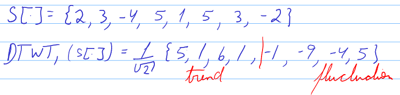
In the penultimate class we learned a little about Stationary DTWT. The idea is that, in theory, when we use Wavelets, they should be linear and invariant in time. However, If we apply two times the DTWT in both the original signal $s[\cdot]$ and a shifted version of it, both results will differ a lot.
As the example he gave us, suppose the signal $s[\cdot] = { 2,3,-4,5,1,5,3,-2}$ is going to be processed via DTWT using Haar filters.
Now if we do the same but shifting the values by one position to the right as in $s_s[\cdot] = { -2,2,3,-4,5,1,5,3}$, the final result is completely different.
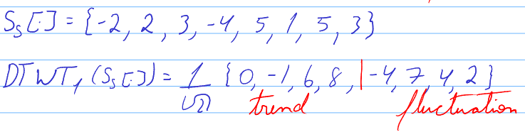
This happens because the mallats algorithm directly applies the downsampling. In that matrix we construct to process signal via Mallat’s algorithm, the two zeros we add at the beggining of each pairs of rows,one is meant to adjust embed the downsampling, so in theory we could remove it, but it would imply a series of different modifications which would cause too much confusion and problems in the meanwhile.
A more elegant solution is to do the following:
- calculate the regular DTWT for $s[\cdot]$
- calculate the same DTWT by for $s_s[\cdot]$
- construct the STDWT based on the coefficients of the results in an specific order
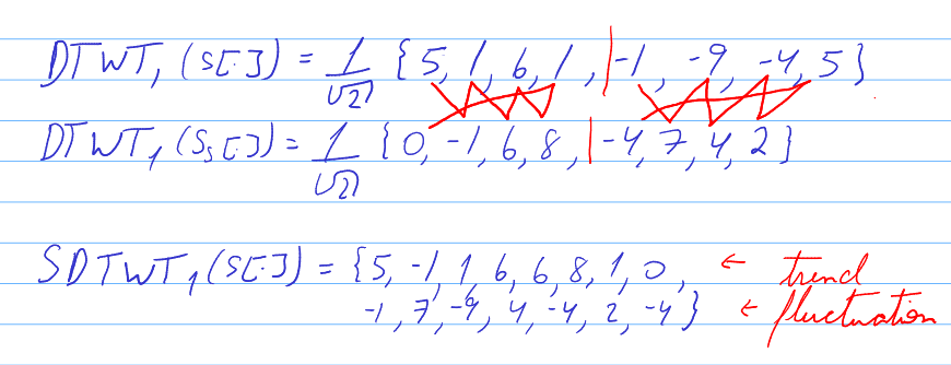
One thing one may notice is that the signal actually has grown, and that’s the what was supposed to happen, since we got rid of the downsampling. The same procedure could be applied in a 2D manner, but it would enlarge the image too much. Even though it’s not usual, I tested it with PyWavelets, which happens to have a function for it.
import os

from PIL import Image
import pywt
import numpy as np
import matplotlib.pyplot as plt

img = Image.open(os.path.join(".", "test.png")).convert("L")

width, height = img.size

new_width = 2 ** int(np.floor(np.log2(width)))
new_height = 2 ** int(np.floor(np.log2(height)))

new_width = max(1, new_width)
new_height = max(1, new_height)

left = (width - new_width) // 2
top = (height - new_height) // 2
right = left + new_width
bottom = top + new_height
cropped_img = img.crop((left, top, right, bottom))

data = np.asarray(cropped_img, dtype=np.float32)
cA, (cB, cC, cD) = pywt.swt2(data, 'haar', level=1)[0]

h,w = cA.shape
quadrants = np.zeros(shape=(2*h,2*w))
quadrants[:h, :w] += cA
quadrants[:h, w:] += cB
quadrants[h:, :w] += cC
quadrants[:h, :w] += cD

fig,ax = plt.subplots(2,1,figsize=(15,20))

ax[0].imshow(cropped_img, cmap="grey")
ax[0].axis("off")
ax[0].set_title("Original Image")

ax[1].imshow(quadrants, cmap="grey")
ax[1].axis("off")
ax[1].set_title("SDTWT_1")
#plt.show()

fig.savefig(os.path.join("..", "processed.png"), bbox_inches="tight")

print("Original Size: ", (new_height, new_width))
print("Processed Quadrant: ", (h,w))
print("Complete Processed size: ", (h*2,w*2))
The script above produce the following image and output.
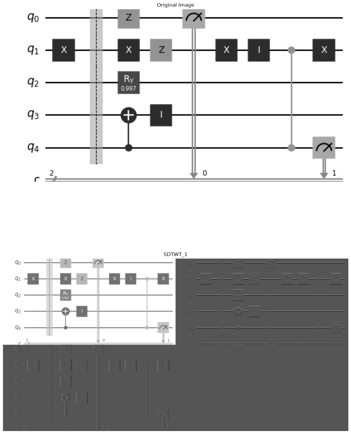
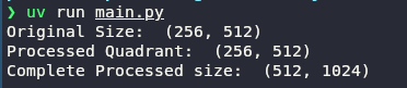
As one can see, the it’s pretty much the same as doing the regular 2D-DWT, however the change is in the size, now the size of each quadrant is the same as the original image and the whole processed matrix is $\times 2$ the size of a regular one. Also, it worth noticing that as the regular procedures we’ve been using, this one also requires the input to be a power of two, that’s why the original image was cropped.
The script above is available in my blog Github repo at https://github.com/Dpbm/personal-blog/tree/main/content/posts/the-processing-tool-nobody-talks-about-P65iteFu0RhKv/sdtwt and can be executed using:
uv sync
uv run main.py
It’s also interesting noticing that calculating the inverse of a SDTWT is as simple as undoing the selection of coefficients and at level 1 calculating the inverse DTWT with the signal.
The last class
The last class was even shorter. It was more like a list of interesting things we could search later.
He gave us a brief overview of Matched Wavelets, DSTs, Curvelets, etc. I’m not risking myself to tell about it since we actually have never used it.
However, there were a moment that I found something really interesting. Our professor was telling us about his PHD thesis. I may actually confuse things a little bit now, but the best I remember of it is that he saying about an experiment he used to create his project on Spikelets. As I understood, the idea was to study filter to get not only use the time frequency domain, but also add another one that brings together with it the shape. I’ll not try to describe it further, sorry! But actually, he showed us the experiment which later I discovered the PHD thesis that from whom created this apparatus and his papers on using it for studying this new kind of filter.
The apparatus consisted on a glued fly on some plastic thing, and in its visual neuron an electrode was connected and processed via an electrical signal and some computers.
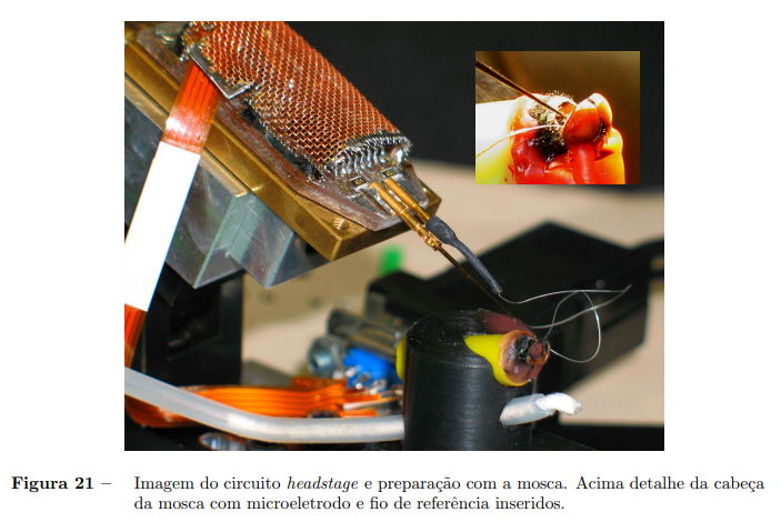
I found it really interesting in fact! I read his paper Nearly symmetric orthogonal wavelets for time-frequency-shape joint analysis: Introducing the discrete shapelet transform’s third generation (DST-III) for nonlinear signal analysis which described it a bit, but I’m not familiar with the thing for now, so I’ll let it for a next post inthe future.
However, I’m listing some interesting papers he showed us at his last class:
- Nearly symmetric orthogonal wavelets for time-frequency-shape joint analysis: Introducing the discrete shapelet transform’s third generation (DST-III) for nonlinear signal analysis
- Instrumentação computacional de tempo real integrada para experimentos com o duto óptico da mosca
- Fusing time, frequency and shape-related information: Introduction to the Discrete Shapelet Transform’s second generation (DST-II)
- Discretewavelet Transform: A Signal Processing Approach
- The Stationary Bionic Wavelet Transform and its Applications for ECG and Speech Processing
- Ripples in Mathematics
- The Curvelet Transform
Beyond the class
Well, in the previous post I also told about the setup for QCOP using wavelets and how everything would work.
In this case, the idea was to create a pipeline like this one:
image --> 2D-DWT level 1 --> sum quadrants 2 and 3 --> enhance sharpness --> binarize (reduce the memory footprint - uint8)
In the real implementation I did something more concise.
Instead of this step by step, I made the kernel do everything at once, and later I decided that the sharpness was not necessary, so the final setup is:
image --> 2dwt kernel --> final image
Kinda nice don’t you think? 🙃
To implement it, I thought about using any fancy stuff, like having my own Cmake setup, some makefiles, conan, whatever, NVCC.
However, Cupy was the best fit for it.
A little tangent in python
I don’t know why but I’m facinated how there’re so many ways to interconnect smoothly.
I always loved how Lua, for example, is so extendable with C. But python sometimes seems even more extendable. You can easily create a module for python using C directly with the Python header. You can use Cython, Jython, PyBind11 if you want to connect with c++, and many other things.
Cupy is another interesting stuff since it’s straight forward to compile kernels and create bridges between your code and your cuda device.
Jax is another insteresting piece of software that can do even more, connecting with TPUs if necessary.
I can’t help loving this kind of integration.
I remember when I was in graduate school, and tried Jython for the first time. I did a simple script to use Java Swing, it was so nice. Unfortunately the sintax was from Python two, even though I liked python2.
from javax.swing import JFrame, JButton, JPanel, JOptionPane
from javax.swing.JOptionPane import showMessageDialog
from java.awt import Dimension, Component, GridBagLayout
from java.awt.event import ActionListener, ActionEvent

class Action(ActionListener):
    def actionPerformed(self,event):
        showMessageDialog(None, "TONTAO :)", "OU",  JOptionPane.INFORMATION_MESSAGE)

f = JFrame("TONTO")
f.setDefaultCloseOperation(JFrame.EXIT_ON_CLOSE)
f.setSize(600,800)

p = JPanel()
p.setLayout(GridBagLayout())


b = JButton("clica aqui tontao")
b.setPreferredSize(Dimension(300, 20))
b.setAlignmentX(Component.CENTER_ALIGNMENT)
b.setAlignmentY(Component.CENTER_ALIGNMENT)

b.addActionListener(Action())

p.add(b)
f.add(p)
f.setVisible(True)
The code above is available at https://raw.githubusercontent.com/Dpbm/faculdade/refs/heads/master/quarto-ano/python/jython-swingera.py.
I never saw a project using Jython for real, and I don’t even know if the Jython project is still being updated. For more familiared people, please leave a comment on that!
I also remember trying to use Brython to do a simple datascience website. I never actually did it, but it seems like the project has evolved a lot. I also saw that there are other attempts to create a thing like Brython but nothing catched my sight anymore in python for web.
Back to the kernels
To create the kernels, I decided to use the following approach. Each pixel in the image would be a thread, so each block would take the maximum amount of threads $1024$ and some indexing tricks would be used to calculate when to apply a filter coefficient or not.

By using this way, it would allow me to easily get the correct pixel and extract the correct value to be applied.
Then, we needed some way to apply the correct coefficients on the pixels. At first, we considered only images of dimensions that were power of two, so I knew that there will be no problems in getting the coefficients in a more generic way.
The way I thought was that, since we use the equation $Y[\cdot\cdot] = m[\cdot][\cdot](s[\cdot][\cdot] \cdot m^{T}[\cdot][\cdot])$ as described in the previous 2D-DWT post, we could use generic coefficients and understand its behavior.
For this project we are using Haar by the way. Since $m[\cdot][\cdot] = m^{T}[\cdot][\cdot]$ for Haar, it was easier to calculate the parts of it.
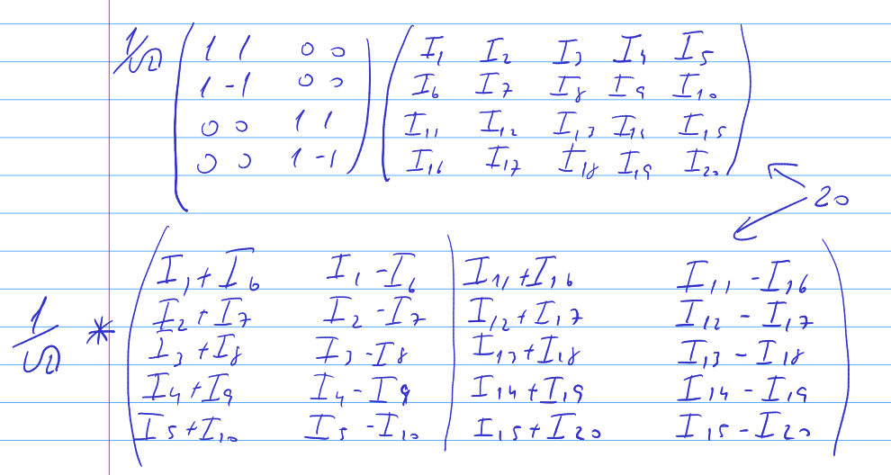
Notice that there’s a pattern forming the the rows and columns. The same happens when applying with $m^{T}$
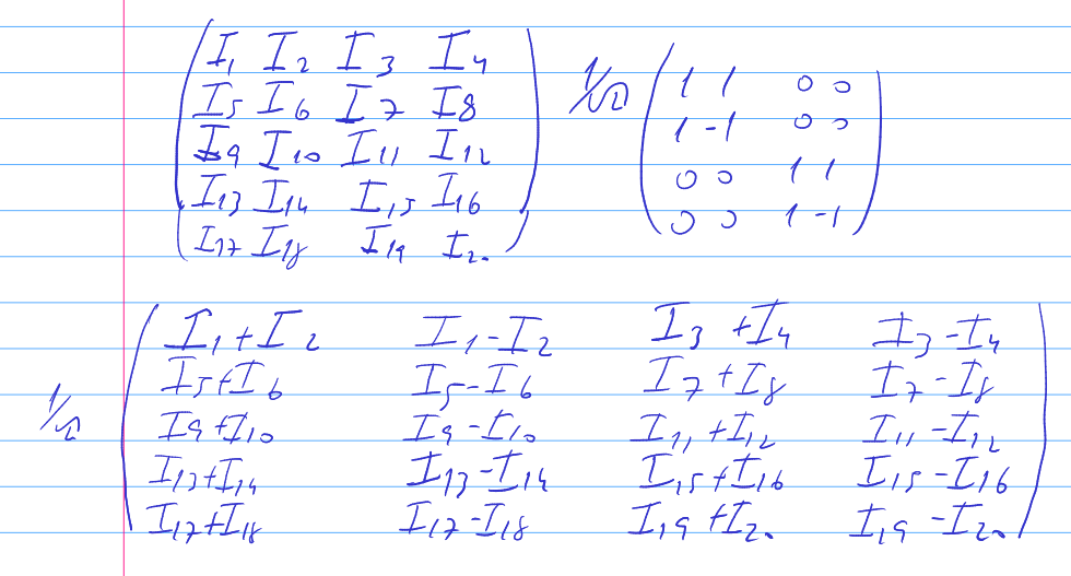
Joining the whole equation.
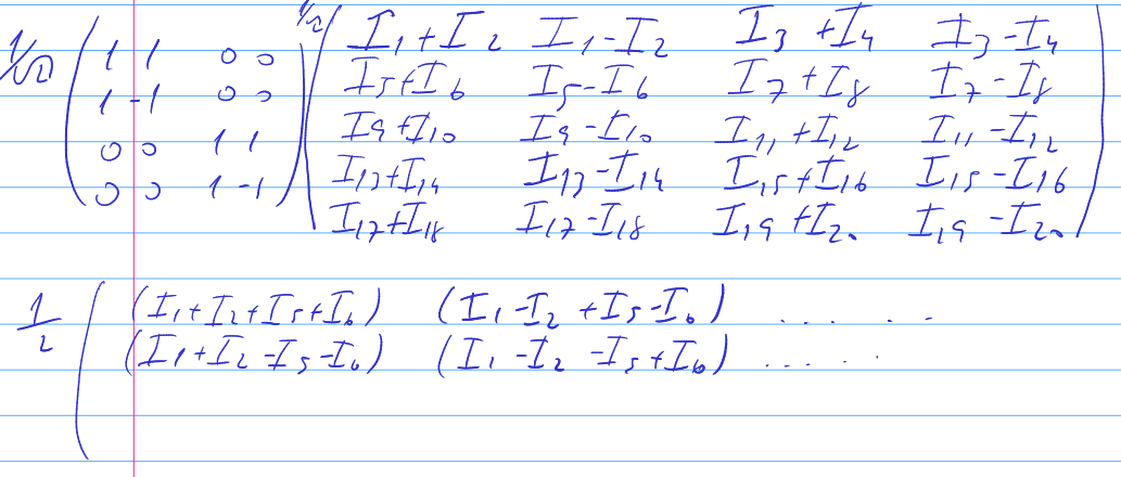
So look that there’s a pattern in how the values are used, this way we can use this information to make or kernel simpler.
What I did was, since each thread could handle $4$ pixels at a time, I don’t need to launch kernels with more than the size of a quadrant, which is half the size of the image.
So at the end, the kernel was only carrying for the quadrant and doing some indexing math I was able to get the correct pixels and generate the images.
The kernel code for the whole image is:
extern "C"{
    __global__ void dtw2(
                    const float* input,
                    float* out,
                    unsigned int quadrant_width,
                    unsigned int quadrant_height,
                    unsigned int img_width,
                    unsigned int max_pixels_quadrant
    ){
        // the total is width*height, being 1024 threads per block
        unsigned int global_index = (blockIdx.x * blockDim.x) + threadIdx.x;
        if(global_index >= max_pixels_quadrant)
            return;

        // indexes based on the threads indexing
        // thinking like half of the image (a quadrant)
        unsigned int width_index = global_index % quadrant_width;   // internal array
        unsigned int height_index = global_index / quadrant_width;  // external array (height/y)

        unsigned int original_img_w_index = width_index * 2;
        unsigned int original_img_h_index = height_index * 2;

        unsigned int curr_input_index = (original_img_h_index * img_width) + original_img_w_index;
        unsigned int curr_input_index_row = ((original_img_h_index+1) * img_width) + original_img_w_index;

        float A_val = 0.5 * (input[curr_input_index] + input[curr_input_index+1] + input[curr_input_index_row] + input[curr_input_index_row+1]);
        float B_val = 0.5 * (input[curr_input_index] - input[curr_input_index+1] + input[curr_input_index_row] - input[curr_input_index_row+1]);
        float C_val = 0.5 * (input[curr_input_index] + input[curr_input_index+1] - input[curr_input_index_row] - input[curr_input_index_row+1]);
        float D_val = 0.5 * (input[curr_input_index] - input[curr_input_index+1] - input[curr_input_index_row] + input[curr_input_index_row+1]);

        unsigned int first_quadrants_row = (height_index * img_width) + width_index;
        unsigned int second_quadrants_row = ((height_index + quadrant_height) * img_width) + width_index;

        out[first_quadrants_row] = A_val;
        out[first_quadrants_row + quadrant_width] = B_val;
        out[second_quadrants_row] = C_val;
        out[second_quadrants_row + quadrant_width] = D_val;
    }
};
The result was amazing!
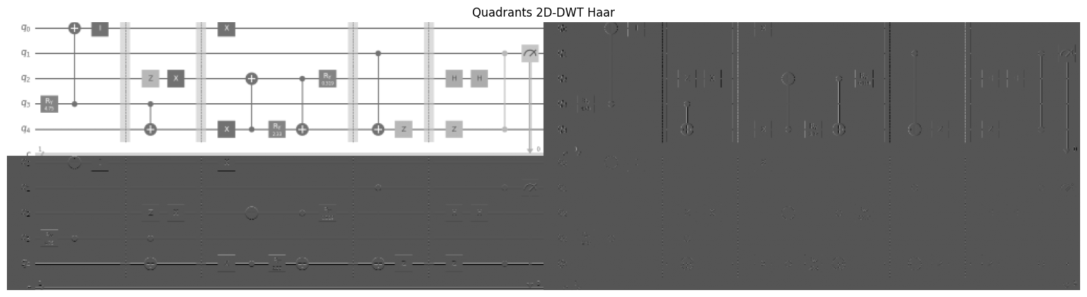
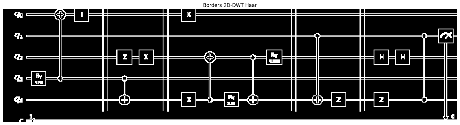
Later, I modified this kernel to care only about the B and C values, and then binarize it by truncation when $pixel < 0.5$.
extern "C"{
    __global__ void dtw2_borders(
                    const unsigned int* input,
                    unsigned char* out,
                    unsigned int quadrant_width,
                    unsigned int img_width,
                    unsigned int max_pixels_quadrant
    ){
        // the total is width*height, being 1024 threads per block
        unsigned int global_index = (blockIdx.x * blockDim.x) + threadIdx.x;
        if(global_index >= max_pixels_quadrant)
            return;

        // indexes based on the threads indexing
        // thinking like half of the image (a quadrant)
        unsigned int width_index = global_index % quadrant_width;   // internal array
        unsigned int height_index = global_index / quadrant_width;  // external array (height/y)

        unsigned int original_img_w_index = width_index * 2;
        unsigned int original_img_h_index = height_index * 2;

        unsigned int curr_input_index = (original_img_h_index * img_width) + original_img_w_index;
        unsigned int curr_input_index_row = ((original_img_h_index+1) * img_width) + original_img_w_index;

        float B_val = 0.5 * (input[curr_input_index] - input[curr_input_index+1] + input[curr_input_index_row] - input[curr_input_index_row+1]);
        float C_val = 0.5 * (input[curr_input_index] + input[curr_input_index+1] - input[curr_input_index_row] - input[curr_input_index_row+1]);
        float sum = abs(B_val + C_val);

        out[(height_index * quadrant_width) + width_index] = (unsigned char) (sum > 0.5 ? 1 : 0);
    }
};
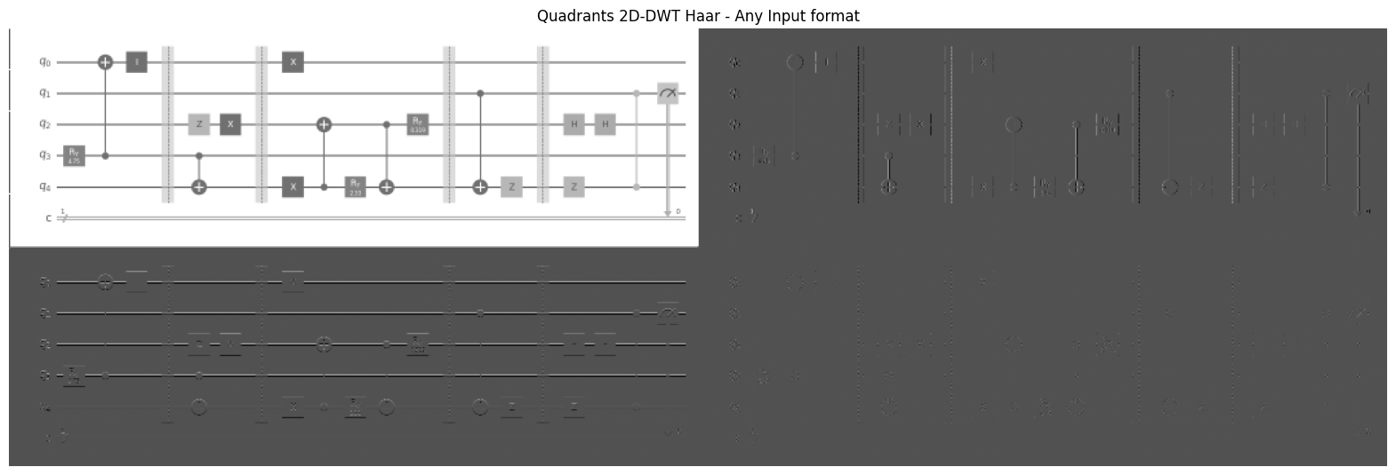
Finally I had to deal with images of arbitrary size. Since padding it would be not the best solution, given that bigger images with a lot of zeros were not something I would like, I added a mechanism to ignore a value (add a zero) in the equation when an index would pass the limits, this way we still has the same size but everything working fine for our case.
extern "C"{
    __global__ void dtw2_any_format(
                    const float* input,
                    float* out,
                    unsigned int quadrant_width,
                    unsigned int quadrant_height,
                    unsigned int img_width,
                    unsigned int max_pixels_quadrant,
                    unsigned int max_pixels_image
    ){
        unsigned int global_index = (blockIdx.x * blockDim.x) + threadIdx.x;
        if(global_index >= max_pixels_quadrant)
            return;

        unsigned int width_index = global_index % quadrant_width;   // internal array
        unsigned int height_index = global_index / quadrant_width;  // external array (height/y)

        unsigned int original_img_w_index = width_index * 2;
        unsigned int original_img_h_index = height_index * 2;

        unsigned int curr_input_index = (original_img_h_index * img_width) + original_img_w_index;
        unsigned int curr_input_index_row = ((original_img_h_index+1) * img_width) + original_img_w_index;

        float current_pixel  = curr_input_index >= max_pixels_image ? 1.0 : input[curr_input_index];
        float next_col_pixel = (curr_input_index+1) >= max_pixels_image ? 1.0 : input[curr_input_index+1];
        float next_row_pixel = curr_input_index_row >= max_pixels_image ? 1.0 : input[curr_input_index_row];
        float diag_pixel     = (curr_input_index_row+1) >= max_pixels_image ? 1.0 : input[curr_input_index_row+1];

        float A_val = 0.5 * (current_pixel + next_col_pixel + next_row_pixel + diag_pixel);
        float B_val = 0.5 * (current_pixel - next_col_pixel + next_row_pixel - diag_pixel);
        float C_val = 0.5 * (current_pixel + next_col_pixel - next_row_pixel - diag_pixel);
        float D_val = 0.5 * (current_pixel - next_col_pixel - next_row_pixel + diag_pixel);

        unsigned int first_quadrants_row = (height_index * img_width) + width_index;
        unsigned int second_quadrants_row = ((height_index + quadrant_height) * img_width) + width_index;

        out[first_quadrants_row] = A_val;
        out[first_quadrants_row + quadrant_width] = B_val;
        out[second_quadrants_row] = C_val;
        out[second_quadrants_row + quadrant_width] = D_val;
    }
};
And the same for binary borders.
extern "C"{
    __global__ void dtw2_borders_any_format(
                    const unsigned int* input,
                    unsigned char* out,
                    unsigned int quadrant_width,
                    unsigned int img_width,
                    unsigned int max_pixels_quadrant,
                    unsigned int max_pixels_image
    ){
        unsigned int global_index = (blockIdx.x * blockDim.x) + threadIdx.x;
        if(global_index >= max_pixels_quadrant)
            return;

        unsigned int width_index = global_index % quadrant_width;   // internal array
        unsigned int height_index = global_index / quadrant_width;  // external array (height/y)

        unsigned int original_img_w_index = width_index * 2;
        unsigned int original_img_h_index = height_index * 2;

        unsigned int curr_input_index = (original_img_h_index * img_width) + original_img_w_index;
        unsigned int curr_input_index_row = ((original_img_h_index+1) * img_width) + original_img_w_index;

        float current_pixel  = curr_input_index >= max_pixels_image ? 1.0 : input[curr_input_index];
        float next_col_pixel = (curr_input_index+1) >= max_pixels_image ? 1.0 : input[curr_input_index+1];
        float next_row_pixel = curr_input_index_row >= max_pixels_image ? 1.0 : input[curr_input_index_row];
        float diag_pixel     = (curr_input_index_row+1) >= max_pixels_image ? 1.0 : input[curr_input_index_row+1];

        float B_val = 0.5 * (current_pixel - next_col_pixel + next_row_pixel - diag_pixel);
        float C_val = 0.5 * (current_pixel + next_col_pixel - next_row_pixel - diag_pixel);
        float sum = abs(B_val + C_val);

        out[(height_index * quadrant_width) + width_index] = (unsigned char) (sum > 0.5 ? 1 : 0);
    }
};
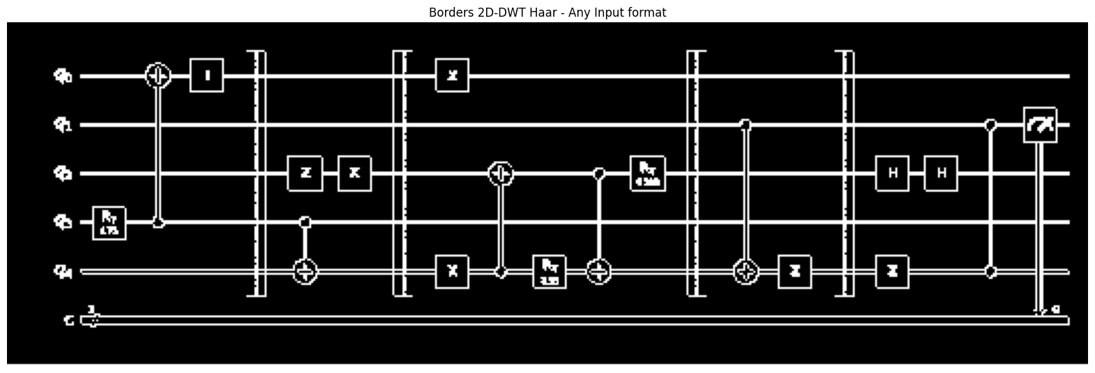
All this code can be seen in the notebook at my QCOP project at https://github.com/Dpbm/qcop/blob/main/notebooks/kernels.ipynb.
Since it was working nicely, I integrated it on my pipeline and recreated the dataset.
    @staticmethod
    def _transform_image(img:Image) -> torch.Tensor:
        """
        Transform and normalize a PIL image into a torch tensor ranging values from 0 to 1.
        """

        img = img.convert("L")

        width,height = img.size
        quadrant_w, quadrant_h = int(np.ceil(width/2)), int(np.ceil(height/2))

        dtw2 = cp.RawKernel(kernel, "dtw2_borders")

        gpu_img = cp.asarray(img,dtype=cp.uint32)
        out = cp.zeros((quadrant_h, quadrant_w), dtype=cp.uint8)

        n_blocks = int(np.ceil((quadrant_h*quadrant_w)/N_THREADS))
        dtw2((n_blocks,), (N_THREADS,), (gpu_img, out, quadrant_w, width, quadrant_h*quadrant_w, width*height))
        cp.cuda.runtime.deviceSynchronize()

        return torch.tensor(out.get())
One thing that was really nice to me was the final dataset size. I was using a H5 file format which was taking almost $24Gb$ a single file.
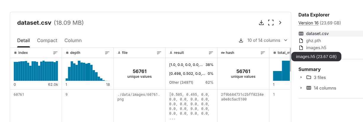
But now the file is less than $2Gb$.
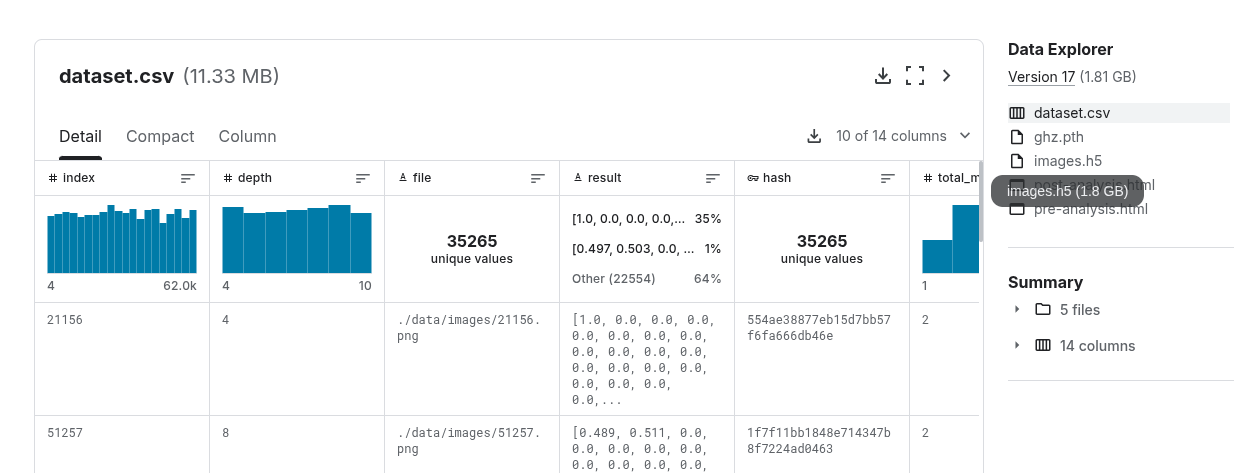
The dataset is available both in my kaggle profile and huggingface at https://www.kaggle.com/datasets/dpbmanalysis/quantum-circuit-images and https://huggingface.co/datasets/Dpbm/quantum-circuits respectively.
I also generate some reports in HTML using Jupyter during the dataset creating, which was nice to have a look on what has happened during the creation and how the data was cleaned.
There’s still a lot of work for this project. I now need to create the vision model, I’m researching it right now. Which models or architectures would you guys recommend me? I thought about using maybe Res-Net or something like that.
Interested readers can reffer to my project at https://github.com/Dpbm/qcop. Feel free to add an issue or open a pull request if you wish 😉.