
These days I’ve been studying a bit about QAOA. It’s been a bit tough to really get the mathematical understanding, since my background is computer science and some mathematical intuition seemed frightening at first, given that I had never heard of trotterizarion and some things like Taylor series or whatever before.
In this article, my goal is to try to explain it in a simple way a computer scientist could understand easily. I’m not here to state that the mathematical portion is not important, but rather to give a more visual and simpler way to understand the goal of each part of the algorithm.
For a more interested reader, I’ll list some papers for a deep diving in the topic at the end.
Since I’m not a specialist, I’m open for comments addressing my mistakes and feel free to share your knowledge as well.
The algorithm
Quantum computing has been a topic of interest for many different fields.
Once the quantum hardware is not ready for large circuits yet, researchers have been applying different hybrid approaches to take advantage of the existing ones.
This hybrid approach levarages variational quantum circuits, which are pretty much circuits that encode some sort of state, and a classical computer is responsible for getting the result, usually the expectation value of the circuit over a Hamiltonian, and based on an optimization procedure the rotation angles of the circuit are updated, repeating the process until a threshold, or a max iterations limit, is reached.
Mathematically, we apply a unitary $U$ with parameters $\theta$ over a quantum state $\ket{\psi_0}$, where $\ket{\psi_0}$ can be any initial state like $\ket{0}^{\otimes{n}}$, such that $U(\theta)\ket{\psi_0} = \ket{\psi(\theta)}$. Then, later we extract the expectation value as $\bra{\psi(\theta)} \hat{H} \ket{\psi(\theta)}$, being $\hat{H}$ the Hamiltonian encoding the problem. Our goal is to minimize the energy of the system, such that our state is the eigenstate which is relative to the minimum, or close, eigenvalue of $\hat{H}$.
This Parametric approach is applied over many different algorithms such as VQE, QAOA, QNN, etc.
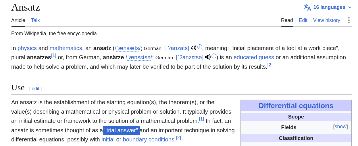
In the general manner, the circuit we use is called ansatz. Taking the definition from wikipedia: https://en.wikipedia.org/wiki/Ansatz, we have that Ansatz is pretty much a “Trial Answer”, i.e. an approximation over a problem.
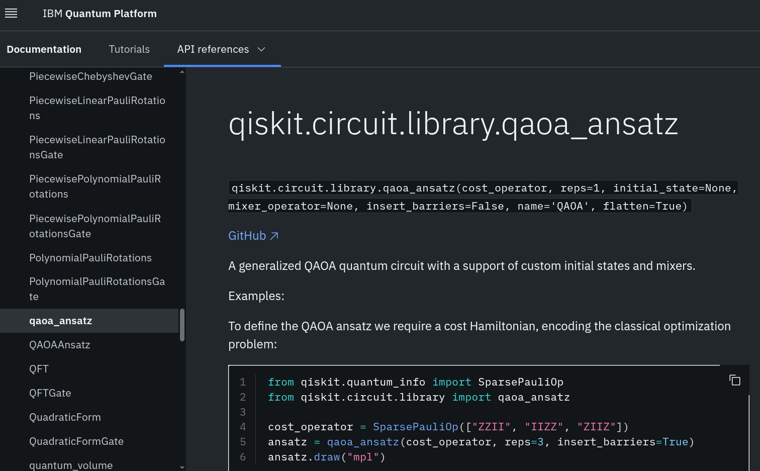
In the literature, there’re many different approaches to generate an ansatz such as EfficientSU2, Real Amplitudes, Evolved Operator Ansatz and also our QAOA Ansatz. In the qiskit library, many of these can be found and used as easily as calling a function or instantiating an object.
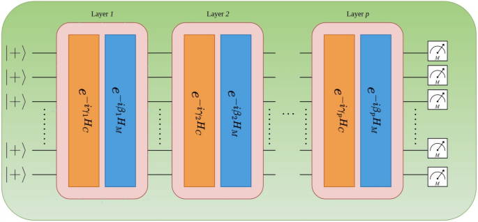
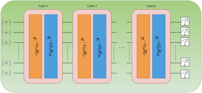
In our case, the QAOA Ansatz is composed of two layers. The first layer encodes the problem based on the Hamiltonian, and the second one, also called as mixer, apply other rotations to explore the search space.
Understanding the structure
In the original paper arXiv:1411.4028, the structure is defined in such a way that applying this combination of layers over and over again $p$ times as $p$ tends to $\infty$, the algoritm is able optimize the problem. For sure it in reality depends on many factors, such as how the Hamiltonian was defined, the way the problem was thought, etc.
For us to understand it more deeply without diving too much in math, let’s look on how the ansatz look like internally. For that, we gonna use the pre-defined ansatz from Qiskit and extract its internals.
from qiskit.quantum_info import SparsePauliOp
from qiskit.circuit.library import qaoa_ansatz

cost_operator = SparsePauliOp(["ZZ"])
ansatz = qaoa_ansatz(cost_operator, reps=1, insert_barriers=False)
ansatz.draw("mpl", filename="../qaoa-circuit-example-1.png")
Using this code, we create a QAOA ansatz with a cost operator (Hamiltonian) which is $\hat{H} = \sigma^{z}_0 \sigma^{z}_1$, applying a Pauli Z operator over both two qubits we have defined.
The final circuit is:
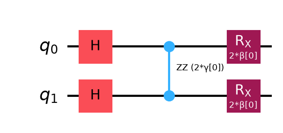
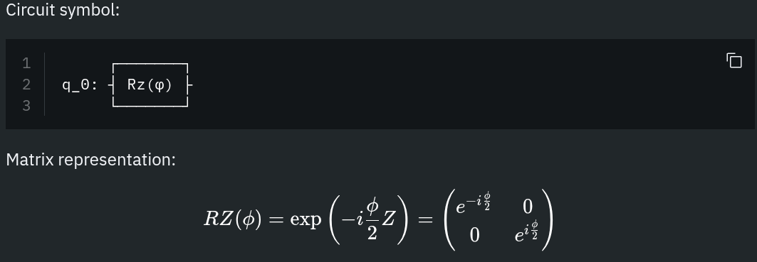
The $ZZ$ gate may seem a bit different for us, so let’s check the documentation.
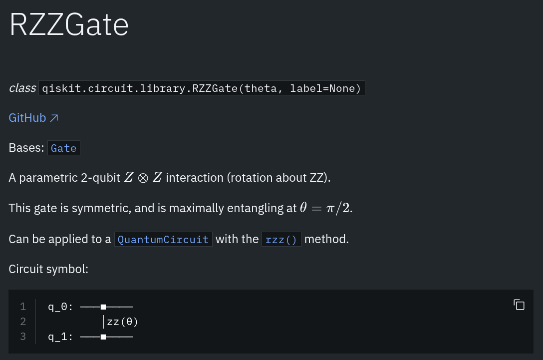
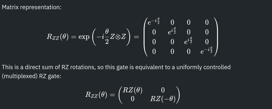
As we presume from the reference, the $RZZ$ is pretty much $RZ$ gates in a different setup, so let’s decompose it to see if we can extract it.
decomposed = ansatz.decompose("rzz")
decomposed.draw("mpl", filename="../qaoa-circuit-example-2.png")
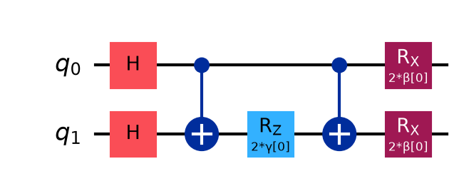
So, the QAOA setup is almost a set of rotations in $Z$ and $X$ based on $\gamma$ and $\beta$ parameters.
One may notice that the parameters are multiplied by $2$. It’s due to the fact that in the original formulation the equations are the following $U(C,\gamma) = e^{-i\gamma C} = \prod_{a=1}^{m} e^{-i\gamma C_a}$ for the cost part, and $U(B,\gamma) = e^{-i\beta B} = \prod_{j=1}^{n} e^{-i\beta \sigma_j^{x}}$ for the mixer. However, the $RZ$ gate applies a phase as $e^{\pm i\frac{\phi}{2}}$, so the multiplication by two comes in order to cancel out with the denominator.
Understanding Bloch Sphere Rotations
Once the QAOA circuit is pretty much a sequence of rotations, we must understand how do they work. The easiest way to understand it is by looking at the Bloch Sphere.
Sometime ago I did a tiny animation on how the rotations look like in the $XYZ$ axis on the Bloch Sphere.
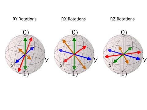
As it can be seen in the video, the rotations work by “rolling” the sphere in one direction. When you rotation in the $X$ axis, for example, you basically fix the $X$ axis and move everything else accordingly.
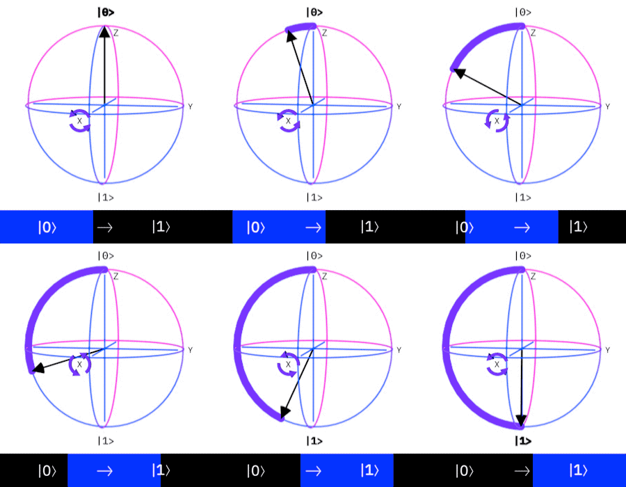
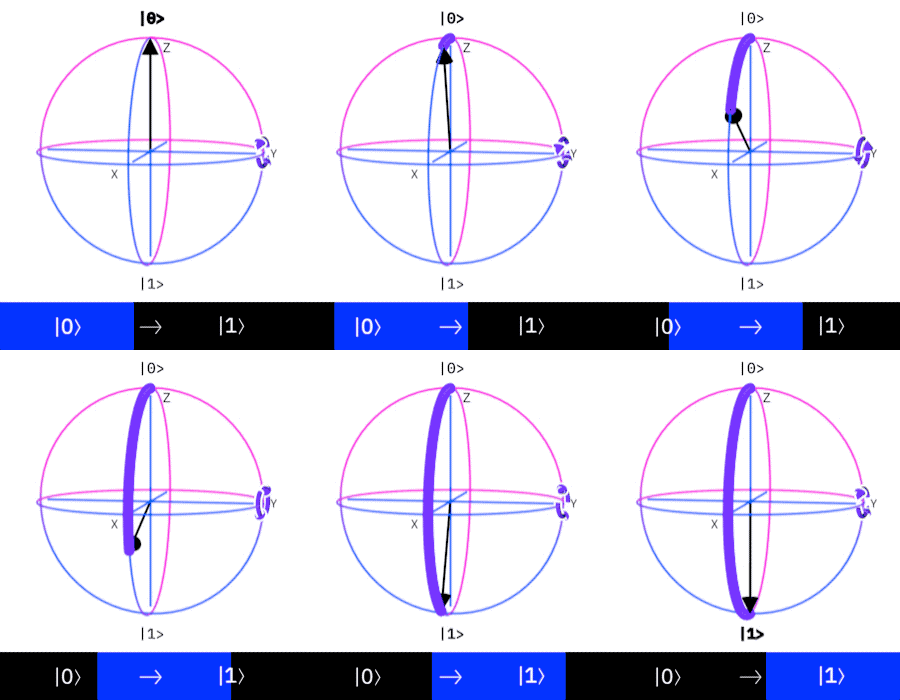
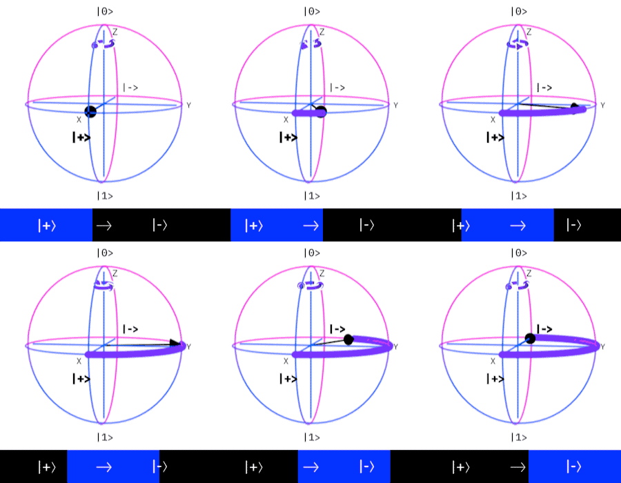
Notice that the rotation in Z has no effect when the state is in the computation basis, so we need to change it to the Hadammard basis before applygin $RZ$ (that’s why QAOA usually start in the $\ket{+}$ state, since this state is an eigen state of $X$, so $RX$ rotations would have no effect directly).
Rotating the state
Ok, now that we have an idea of it, lets do a simple test. How does it look like in a single qubit setup?
For this test, we set a single qubit QAOA with Hamiltonian $\hat{H} = \sigma^{z}_0$, which creates the circuit:
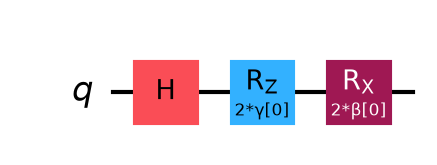
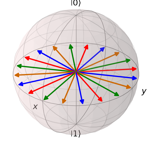
Let’s first find out what happens when we perform the $RZ$ rotations in the Hadammard axis.
from qiskit.quantum_info import Statevector
from qiskit.circuit.library import RZGate
from qutip import Bloch, Qobj

import numpy as np

angles = np.arange(0, 2*np.pi, np.pi/10)

states = []
for angle in angles:
    # start in the X axis
    state = Statevector.from_label("+")

    # apply the RZ gate with the angle
    state = state.evolve(RZGate(angle))

    # save the state
    states.append(Qobj(state.data))


bloch = Bloch()
bloch.add_states(states)
bloch.save("../bloch-rz-rotations.png")
Using the Qutip library we can add all the possible states in the Bloch Spehre and compare were they can appear.
Now, let’s compare with what happens when we apply a single rotation in $X$ with angle $\pi/2$ after $RZ$.
from qiskit.circuit.library import RXGate

states2 = []
for angle in angles:
    # start in the X axis
    state = Statevector.from_label("+")

    # apply the RZ gate with the angle
    state = state.evolve(RZGate(angle))

    # apply the RX gate with the fixed angle pi/2
    state = state.evolve(RXGate(np.pi/2))

    # save the state
    states2.append(Qobj(state.data))

bloch = Bloch()
bloch.add_states(states2)
bloch.save("../bloch-rz-rx-rotations.png")
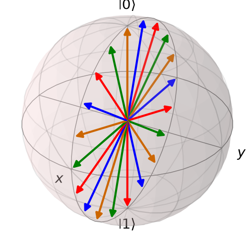
It maps the values back to $Z$, so we can get our states in the computation basis again.
It seems like a mix of something interesting and strange at the same time, but it’s the effect of rotation accross perpendicular axis.
In general, that’s how QAOA can approximate your solution. By applying a succession of rotations and then calculating the expectation value. The general idea is that the transformed state $\ket{\psi(\theta)}$ gets close to the eigenstate of smallest energy of our $\hat{H}$. Once our Hamiltonian is $\hat{H} = \sigma^{z}_0$, we know that the solution we are searching $\langle \hat{H} \rangle = -1$, since our Hamiltonian encodes a single $Z$ operator that has minimum eigenvalue $-1$, so the state we want to reach is $\ket{1}$, which explains this remapping between $X$ to $Z$ axis.
Given this toy model, our goal was to map the circuit $\ket{\psi} \to \ket{1}$, reaching the minimum value and optimizing our “problem”.
Different setups with $I \otimes Z$
As a final experiment, let’s check what happens when we use identity operators within our cost Hamiltonian.
cost_operator_3 = SparsePauliOp(["I"])
ansatz = qaoa_ansatz(cost_operator_3, reps=1, insert_barriers=False)
ansatz.draw("mpl", filename="../qaoa-circuit-example-4.png")

cost_operator_4 = SparsePauliOp(["ZI"])
ansatz = qaoa_ansatz(cost_operator_4, reps=1, insert_barriers=False)
ansatz.draw("mpl", filename="../qaoa-circuit-example-5.png")

cost_operator_5 = SparsePauliOp(["IZ"])
ansatz = qaoa_ansatz(cost_operator_5, reps=1, insert_barriers=False)
ansatz.draw("mpl", filename="../qaoa-circuit-example-6.png")
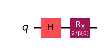
For this case, where $\hat{H} = I_{0}$, no $RZ$ is used, given the matrix exponential, we would have the $I$ with some global phase, so actually nothing happens. This way we can eliminate the first part and keep only the mixer. However, once $\ket{+}$ is an eigen state of $X$, we know that nothing would happen with any possible $\beta$ value applied on this, only a few changes in phase and nothing else.
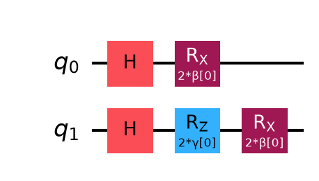
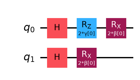
Now for two qubits, notice that these two examples have no $CNOT$ gates, once their Hamiltonian is only applied for local cost of single qubits. In the $ZZ$ example, we were adding a relation between qubits $0$ and $1$, so the $CNOTs$ were used to apply this correlation in form of entanglement.
References
For more details on the algorithms:
- A Quantum Approximate Optimization Algorithm
- An Introduction to the Quantum Approximate Optimization Algorithm
- Mixer Hamiltonian with QAOA for Max k-coloring : numerical evaluations
The code examples shown here are available at: https://github.com/Dpbm/personal-blog/tree/main/content/posts/qaoa-the-simple-way-KKX4DYGABJWBM/reverse-qaoa.
To run it, use:
uv sync
uv run main.py